In this post I will describe a technique I have been applying at Kunumi to explain the output of Deep Neural Networks trained to solve Natural Language Processing (NLP) problems.

Some of the diagrams and part of the Jupyter Notebook examples presented here are based on the excellent set of tutorials by Ben Trevett, released under the MIT license.

Deep Learning applied to Natural Language Processing

Over the last 5 years, Deep Learning has become an essential ingredient of state-of-the-art NLP models.

Wikipedia defines NLP as “…a subfield of computer science, information engineering, and artificial intelligence concerned with the interactions between computers and human (natural) languages…”.

Practically, NLP today focuses on creating Machine Learning models capable of understanding specific aspects of text, such as sentiment analysis, part-of-speech tagging, named entity recognition, language translation, etc.

“Deep Learning” refers to the application of Deep Neural Networks usually trained using Stochastic Gradient Descent. The Neural Networks most frequently applied to NLP problems are Recurrent Neural Network (RNN) variants (such as LSTM and GRU) and Convolutional Neural Networks (CNN). Although RNNs are a natural fit for NLP problems due to their sequential data processing nature, CNNs are increasingly being adopted in the field as they provide essentially the same level of accuracy at a fraction of the processing cost.

Interpreting Deep Neural Network outputs

Over the last couple of years, models transitioned from prototyping to production. Because of that, model interpretation has started to receive a lot of interest due to the importance of understanding and justifying the probability distributions generated as the output of these models.

When talking about model interpretation one usually means to obtain some kind of explanation for a particular output of a Machine Learning model. This explanation is usually framed in terms of the input features: one would like to see some evidence in the input features that justify the model predictions.

Neural Networks have been traditionally seen as uninterpretable black-boxes by the Machine Learning community. However, many new techniques have been developed in order to try to understand the information processed by these models. Techniques such as gradients, LIME, GuidedBackProp, and Layer wise relevance propagation (LRP), among others, provide ways to identify relevant input features by analyzing how information propagates inside Neural Networks.

The gradients technique will be the focus of this post. This technique uses the information contained in the gradients generated during the backward pass of the backpropagation algorithm as a proxy for feature importance. Even though it does not always yield the most interpretable explanations it is straightforward to implement and computationally inexpensive when compared to the other methods.

Gradient-based model explanations

The backpropagation algorithm used to train modern Neural Networks has two phases: forward and backward. In the forward phase, the input signal is propagated through the layers of the network until an output layer is reached. A loss function is then used to compute the error between the network output and the ground truth (label).

In supervised learning, this loss function is differentiable and therefore can produce a gradient, which can be used to correct the weights of the last layer of the Neural Network in order to make the output closer to the ground truth. Since every signal transformation performed by the neural network during the forward pass is also differentiable, the gradient of the output with regard to the error can be used to compute a gradient for the last layer, then of the penultimate layer, then of the layer before that and so on until reaching the input signal. These gradients are then used to make a small update to every weight of the Neural Network. Illustration of the forward and backward passes. Source: http://www.cnblogs.com/daniel-D/archive/2013/06/03/3116278.html

The gradients of the error with regards to the input are usually ignored, as the input is not updated by the backpropagation algorithm. However, these gradients still provide some very useful information: they describe how each signal component in the input would need to change in order to make the network output closer to the label.

The way backpropagation shapes the neural network during training makes it so that uninteresting parts of the input signal get less gradient signal than interesting ones. Thus, measuring the magnitude of the gradients received by each input feature during a backward pass with regard to a specific output can be used as a proxy to how important this feature is to the identification of the label under consideration.

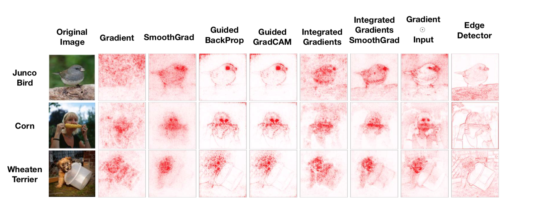A compairson of different explanation methods for visual classification. Most of the methods are based on the interpretation of the backpropagation gradients. Source: “Sanity Checks for Saliency Maps” https://arxiv.org/abs/1810.03292

As the above figure shows, the gradient information by itself seldom generates understandable explanations of classification on images. Some post-processing of these gradients is needed in order to turn them into meaningful salience maps. Nevertheless, they provide the easiest way to get some explanation about the reasoning of a deep learning model.

Deep Learning in NLP

Most of the work developed in feature interpretation for Deep Neural Networks using gradient information has been done in the context of processing images. The focus is usually in identifying regions of an input image most relevant for classification in a particular class. In order to understand how to adapt these methods to work with textual input, we need to understand first how natural language is usually represented as input to a Deep Neural Network.

Word Vector Representation

Natural language documents are sequences of sentences, which in turn are themselves sequences of words that in their turn are sequences of syllables (n-grams) that can be broken down into individual characters. An NLP model usually makes some simplification by looking at natural language at a specific zoom level, ignoring the lower-level components. Even though there are NLP models that work at the character or n-gram level, most models work at the word level.

Once you choose to look at the input word by word, you still need to choose a way to represent each word. There are many ways to do that but, in the Deep Learning community, one particular way became the de-facto standard for that task: word vectors.

Since their first publication in 2013, word vectors have taken the Deep Learning world by storm. This representation model each word as a multi-dimensional feature vector. The vector representation for each word is jointly learned from a large corpus of text in an unsupervised way by a neural network solving an auxiliary prediction task such as phrase completion. After training the original neural network is discarded and only the internal representation it has learned for each word is kept. It has been demonstrated that this representation contains syntatcic and semantic information about each word.

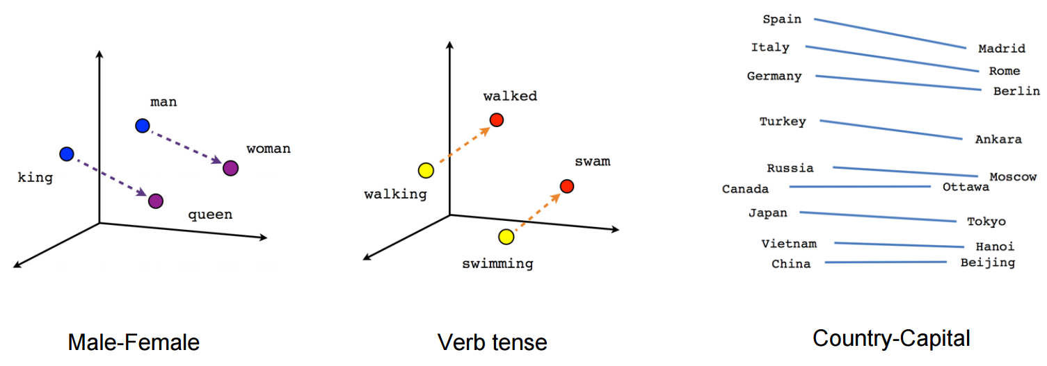Word vectors capture semantic information. This can be demonstrated by using them to solve analogy tasks such as: King-Man+Woman=Queen. Source: https://www.tensorflow.org/images/linear-relationships.png

Word2Vec is the original word vector learning technique. There are currently other learning techniques such as Glove and FastText. All these techniques learn semantically signifficant multi-dimensional word embeddings and therefore are considered equivalent from the point of view of this post.

Phrase-level representation with word vectors

In NLP one is usually not interested in interpreting individual words. The units of interest are phrases, paragraphs, and documents. Therefore, it is necessary to find a way of combining word vectors into higher-level representations. Many different techniques for solving this particular problem are under development. In this post, we will focus on the most common one which is simply word vector concatenation.

In this technique, the phrase representation is constructed by concatenating the word vector representing each word. Word vectors are usually high-dimensional, usually having 300 dimensions or more. We can imagine the word vectors as being piled up on top of one another forming a structure aking to an image:

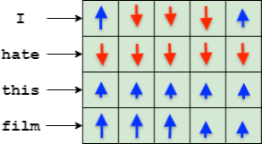
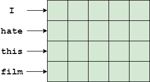An example of a phrase represented as a concatenation of word vectors

Assuming our word vectors have 300 dimentions, the phrase “I hate this film” can be represented as an image of 300x4 “pixels”, where each line of the image corresponds to a word and each column to a word vector feature. A convolutional network can then be used to process this representation using the same standard convolutional blocks used in image processing. Alternatively, a recurrent neural network can process the same data line-by-line as part of a sequence model.

Explaining Deep NLP model decisions

A first gradient interpretation attempt

We already saw how the gradient information generated by backpropagation can be used to generate interpretations for images. Since the word vector sequence representation described above is essentially equivalent to an image, can we also use gradients to generate interpretations of Deep NLP model outputs?

It turns out we can but, in order to do that, we need to understand how the semantic properties of word vectors interact with the gradient information. Let’s look into an example.

All the code in this example is available in this Collaboratory notebook. This notebook implements a deep convolutional NLP module for sentiment analysis in Pytorch. A version using a recurrent neural network is also available.

Suppose we are creating a neural network for movie sentiment analysis. We train the network using the IMDB movie review dataset. After training we submit the following phrase to be analyzed:

“I loved this movie, but the main actor sucks.”

(I know. Ambiguous review. The Matrix, right? )

We get the following prediction from the model: 0.877.

Not bad: the model gives a probability of 88% that this is a positive phrase in a movie review, even though the phrase itself contains both positive elements (related to the film) and negative elements (related to the main actor in the film).

Why does the model think that this is a positive phrase? In order to answer that we need to obtain an explanation. Using the gradient method, we will try to explain this phrase as follows:

1. Run a forward() pass on the neural network with this phrase as input
2. Compute the loss (we would expect the output to be 100% so there is still room for improvement here)
3. Run a backward() pass and collect the gradients of the loss w.r.t the input
4. For each word vector in the input, compute the norm of the corresponding gradient vector. This measures the amount of gradient received by each input word.
5. Since we want to compare one word against another, we normalize each word gradient norm by the maximum gradient norm.

If we do that, we obtain the following:

I (0.525) loved (1.000) this (0.580) movie (0.588) , (0.155) but (0.000) the (0.032) main (0.114) actor (0.196) sucks (0.400) . (0.136)

The number to the right of each word is the (relative) gradient norm received by the corresponding word vector. If we interpret that number as a measure of how much “focus” the neural network is giving to each word, we can see that it is focusing more in the “I loved this movie” part than in the “but the main actor sucks” part, which justifies the 88% positive probability score.

We can also notice that the word “sucks” gets a relatively high amount of focus compared to the other words in the second half of the sentence. Why does that happen?

Useful as the gradient module information is, it does not provide information about how the neural network is interpreting a particular word it is focusing on. But it is possible to get that information if we dig deeper into the meaning of word vector dimensions and how they interact with the gradient.

A better semantic interpretation

Ideally, we would like to understand not only which words the model is focusing on, but also why the model is focusing on these specific words. Let’s see if it is possible to use gradient information for that.

The main idea we need to keep in mind is this: due to the use of the word vector representation, the neural network sees each word not as a discrete entity but as a set of continuous attribute values. Since word vectors are learned through unsupervised learning, it is difficult to assign a specific interpretable meaning to each dimension. However, world analogy tasks demonstrate that these dimensions encode semantic meaning. There can be, for instance, a dimension (or subset of dimensions) that encode “polarity” (where larger values correspond to more positive words). There may be dimensions that encode the function of the word (noun, verb, article etc.). The point is that each word is seen as a multi-dimensional object containing different quantities of each possible attribute.

Looking at an individual word vector dimension we see that the gradient applied to it describes a way in which this specific dimension should be transformed in order to minimize the loss function. This transformation can be decomposed in two components: a direction (increase or decrease) and a magnitude. Each individual word vector dimension receives a different gradient and we can imagine the complete gradient information received as specifying a vector transformation that would modify the original word vector in the direction of a “better” word relative to the loss of the chosen class.

Given all that, we can think about a new way of constructing an explanation based on the gradients:

1. Run a forward pass
2. Compute the gradient of the loss w.r.t the desired output
3. Run a backward() pass and collect the gradients of the loss w.r.t the input

4. For each word vector in the input, compute the magnitude change as follows:

   4.1 Let W be the original word vector and gradW be the gradient of this vector w.r.t the loss.

   4.2 Compute Wmod = W-gradW (this is equivalent to a SGD step)

   4.3 Compute the magnitude change: WChange = norm(W)-norm(Wmod)

5. Compute the mean (WChangeMean) and variance (WChangeVar) of the magnitude changes for the entire phrase or document.
6. For each word, compute the word explanation score: WScore=(WChange-WChangeMean)/WChangeVar

The algorithm described above assumes that the magnitude of the change in the word vector can be used to capture the direction in which a word would change if SGD used the corresponding gradient to optimize its vector. If the magnitude shrinks we interpret it as the word being “disliked” by the neural network (in the context of the other words present and the desired output). This is simple to understand: if the magnitude shrinks that means there are significant dimensions of the word that are being “erased” by the gradient in order to improve the loss function. On the other hand, an increase in magnitude for the word vector means that some dimensions are being enhanced by the gradient, so we interpret that as the word being “liked” by the network.

The steps 5 and 6 of the algorithm were developed experimentally and corresponding to using the z-score of the word vector magnitude change. I found in practice that using the z-score provides a more interpretable explanation than using the absolute magnitude change because the gradient of a single backward pass is usually very small.

Let’s look at our test phrase interpretation using this new method:

I (-0.794) loved (2.460) this (0.736) film (0.274) , (-0.576) but (-0.168) the (-0.143) main (-0.022) actor (-0.457) sucks (-1.448) . (0.138)

This looks much better and at the same time intriguing. We can now see that the network is indeed focusing on the “loved” word and that it wants to see more of it in order to improve the loss. Since we are improving the loss relative to the positive class, we can interpret any word with a positive z-score as “positive”.

We can also see that the word sucks is a “negative” word in this context, since the gradient is aiming to “erase” it (not as much as it wants to enhance the word “love” tough).

The intriguing part it the word ‘I’. The network seems to dislike it more than any other word except “sucks”. Is that a real effect or an artifact of the gradient computation? We can try to answer that by removing the word ‘I’ from the phrase:

loved (1.976) this (0.404) film (-0.070) , (-0.273) but (-0.060) the (-0.018) main (0.200) actor (-0.519) sucks (-2.084) . (0.445) : 0.542

Oops. Only 54.2% probability of positive. The network certainly misses some aspects of the word ‘I’, even though it dislike others. Let’s try to replace it for a different pronoun:

We (-0.324) loved (2.485) this (0.709) film (0.233) , (-0.642) but (-0.222) the (-0.196) main (-0.072) actor (-0.521) sucks (-1.543) . (0.094) : 0.884

We can see from the word score and output probability that the model likes ‘We’ a little better than ‘I’. But it still doesn’t like something about ‘We’. Let’s change it for a very different word:

Fans (1.127) loved (2.173) this (0.521) film (0.074) , (-0.742) but (-0.350) the (-0.326) main (-0.210) actor (-0.629) sucks (-1.584) . (-0.055) : 0.894

The word ‘Fans’ is better from the model point of view than ‘We’ to replace ‘I’ in order to improve the output probability score for the positive class.

Certainly, the best thing we can do to improve the “positiveness” of the phrase would be to remove the word “sucks”:

Fans (1.058) loved (2.279) this (0.433) film (-0.068) , (-0.981) but (-0.622) the (-0.580) main (-0.381) actor (-0.654) . (-0.486) : 0.949

The explanations generated by this method sure seem to be useful for providing a better human-level understanding of how the input features (words) are being interpreted in the context of this classification problem.

I have successfully applied this technique to different types of classification problems using different types of neural network architectures, with similar results.

In my next blog post, I will continue to explore this topic and provide further evidence for the validity of this interpretation of gradients by creating an algorithm that can rewrite phrases in a way that moves the model output in the desired direction (positive or negative).